17 Poisson Regression
This chapter is under heavy development and may still undergo significant changes.
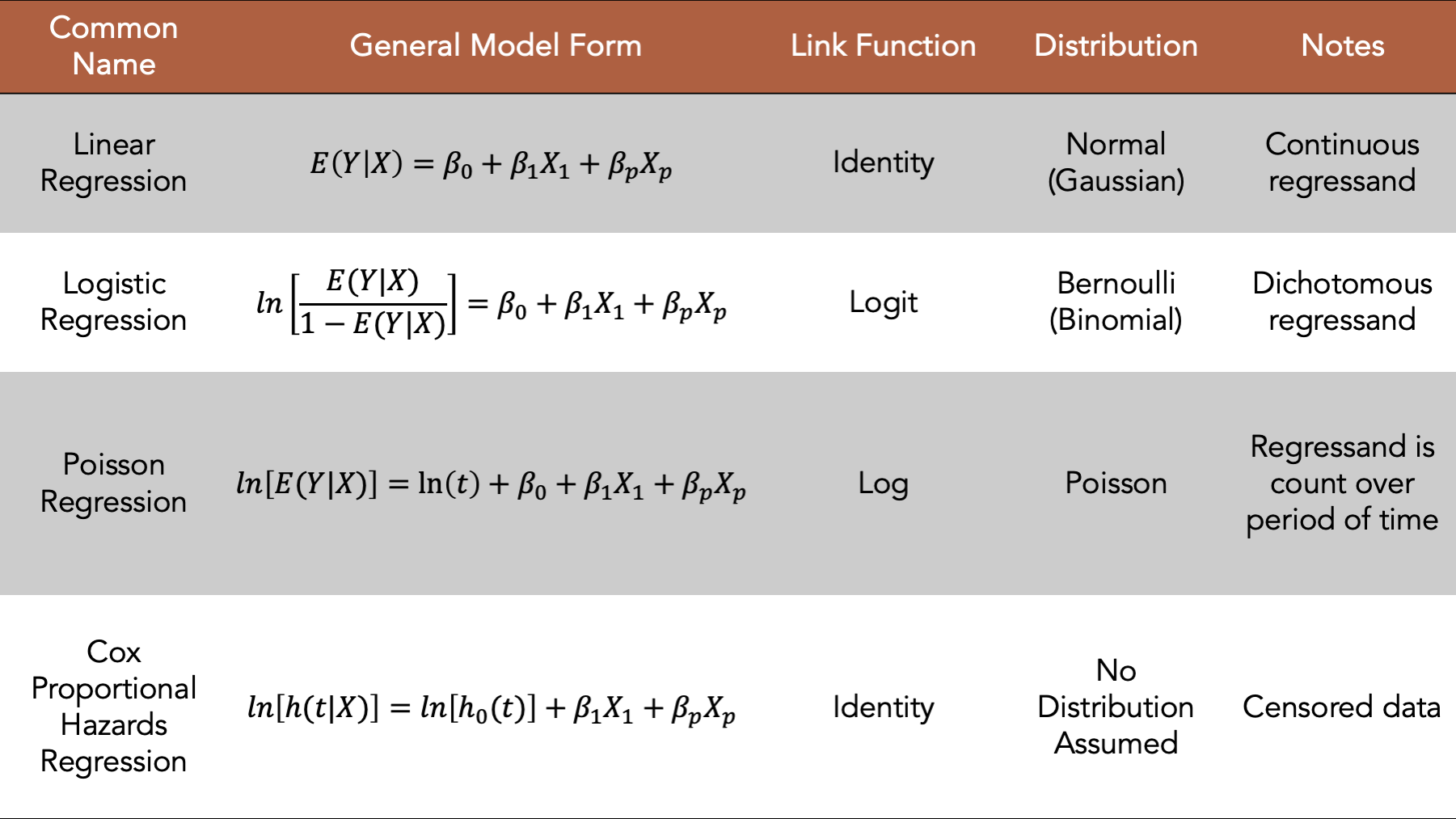
Figure 17.1: Four commonly used generalized linear models.
We introduced regression modeling generally in the introduction to regression analysis chapter. In this chapter, we will discuss fitting Poisson regression models, a type of generalized linear model, to our data using R. In general, the Poisson model is a good place to start when the regressand we want to model contains counts. We will begin by loading some useful R packages and simulating some data to fit our model to. We add comments to the code below to help you get a sense for how the values in the simulated data are generated. But please skip over the code if it feels distracting or confusing, as it is not the primary object of our interest right now.
# Load the packages we will need below
library(dplyr, warn.conflicts = FALSE)
library(broom) # Makes glm() results easier to read and work with
library(ggplot2)
library(meantables)
library(freqtables)
# Set the seed for the random number generator so that we can reproduce our results
set.seed(123)
# Set n to equal the number of people we want to simulate. We will use n
# repeatedly in the code below.
n <- 20
# Simulate a data frame with n rows
# The variables in the data frame are generic continuous, categorical, and
# count values. They aren't necessarily intended to represent any real-life
# health-related state or event
df <- tibble(
# Create a continuous regressor containing values selected at random from
# a normal distribution
x_cont = rnorm(n, 10, 1),
# Create a categorical regressor containing values selected at random from
# a binomial distribution with a 0.3 probability of success (i.e.,
# selecting a 1)
x_cat = rbinom(n, 1, .3),
# Create a continuous regressand that has a value that is equal to the value
# of x_cont plus or minus some random variation. The direction of the
# variation is dependent on the value of x_cat.
y_cont = if_else(
x_cat == 0,
x_cont + rnorm(n, 1, 0.1),
x_cont - rnorm(n, 1, 0.1)
),
# Create a categorical regressand that has a value selected at random from
# a binomial distribution. The probability of a successful draw from the
# binomial distribution is dependent on the value of x_cat.
y_cat = if_else(
x_cat == 0,
rbinom(n, 1, .1),
rbinom(n, 1, .5)
),
# Create a regressand that contains count data selected at random from
# a categorical distribution. The probability of a selecting each value from
# the distribution is dependent on the value of x_cat.
y_count = if_else(
x_cat == 0,
sample(1:5, n, TRUE, c(.1, .2, .3, .2, .2)),
sample(1:5, n, TRUE, c(.3, .3, .2, .1, .1))
)
)
# Print the value stored in df to the screen
df## # A tibble: 20 × 5
## x_cont x_cat y_cont y_cat y_count
## <dbl> <int> <dbl> <int> <int>
## 1 9.44 0 10.5 0 5
## 2 9.77 0 10.7 0 2
## 3 11.6 0 12.6 0 5
## 4 10.1 0 11.2 0 3
## 5 10.1 0 11.2 0 4
## 6 11.7 0 12.8 0 2
## 7 10.5 0 11.5 0 3
## 8 8.73 0 9.73 0 4
## 9 9.31 0 10.3 0 1
## 10 9.55 1 8.53 0 1
## 11 11.2 0 12.2 0 3
## 12 10.4 0 11.3 0 2
## 13 10.4 1 9.43 1 1
## 14 10.1 0 11.3 0 4
## 15 9.44 0 10.6 0 1
## 16 11.8 0 12.7 0 2
## 17 10.5 0 11.5 0 2
## 18 8.03 1 7.03 1 2
## 19 10.7 1 9.61 1 5
## 20 9.53 0 10.5 0 417.1 Count regressand continuous regressor
Now that we have some simulated data, we will fit and interpret a few different Poisson models. We will start by fitting a Poisson model with a single continuous regressor.
glm(
  y_count  ~ x_cont,                # Formula
  family   = poisson(link = "log"), # Family/distribution/Link function
  data     = df                     # Data
)
##
## Call: glm(formula = y_count ~ x_cont, family = poisson(link = "log"),
## data = df)
##
## Coefficients:
## (Intercept) x_cont
## 0.44666 0.05734
##
## Degrees of Freedom: 19 Total (i.e. Null); 18 Residual
## Null Deviance: 13.74
## Residual Deviance: 13.57 AIC: 73.74This model isn’t the most interesting model to interpret because we are just modeling numbers without any context. However, because we are modeling numbers without any context, we can strip out any unnecessary complexity or biases from our interpretations. Therefore, in a sense, these will be the “purist”, or at least the most general, interpretations of the regression coefficients produced by this type of model. We hope that learning these general interpretations will help us to understand the models, and to more easily interpret more complex models in the future.
17.2 Count regressand categorical regressor
Next, we will fit a Poisson model with a single categorical regressor. Notice that the formula syntax, the distribution, and the link function are the same for the single categorical regressor as they were for the single continuous regressor We just swap our x_cont for x_cat in the formula.
glm(
  y_count  ~ x_cat,                 # Formula
  family   = poisson(link = "log"), # Family/distribution/Link function
  data     = df                     # Data
)
##
## Call: glm(formula = y_count ~ x_cat, family = poisson(link = "log"),
## data = df)
##
## Coefficients:
## (Intercept) x_cat
## 1.0776 -0.2666
##
## Degrees of Freedom: 19 Total (i.e. Null); 18 Residual
## Null Deviance: 13.74
## Residual Deviance: 13.17 AIC: 73.3317.2.1 Interpretation
Intercept: The natural log of the mean of
y_countwhenx_catis equal to zero.x_cat: The average change in the natural log of the mean of
y_countwhenx_catchanges from zero to one.
Now that we have reviewed the general interpretations, let’s practice using logistic regression to explore the relationship between two variables that feel more like a scenario that we may plausibly be interested in.
17.3 Number of drinks and personal problems example
Consider a study with the following questions:
“The last time you drank, how many drinks did you drink?”
“Sometimes people have personal problems that might result in problems with work, family or friends. Have you had personal problems like that?”
set.seed(100)
n <- 100
drinks <- tibble(
  problems = sample(0:1, n, TRUE, c(.7, .3)),
  age = rnorm(n, 50, 10),
  drinks = case_when(
    problems == 0 & age > 50 ~ sample(0:5, n, TRUE, c(.8, .05, .05, .05, .025, .025)),
    problems == 0 & age <= 50 ~ sample(0:5, n, TRUE, c(.7, .1, .1, .05, .025, .025)),
    problems == 1 & age > 50 ~ sample(0:5, n, TRUE, c(.2, .3, .2, .2, .05, .05)),
    problems == 1 & age <= 50 ~ sample(0:5, n, TRUE, c(.3, .1, .1, .2, .2, .1)),
  )
)

drinks
## # A tibble: 100 × 3
## problems age drinks
## <int> <dbl> <int>
## 1 0 45.5 0
## 2 0 32.6 0
## 3 0 51.8 5
## 4 0 69.0 0
## 5 0 27.3 1
## 6 0 59.8 4
## 7 1 36.0 0
## 8 0 68.2 0
## 9 0 63.8 0
## 10 0 41.6 0
## # ℹ 90 more rows17.3.1 Count regressand and continuous regressor
## [1] 1.06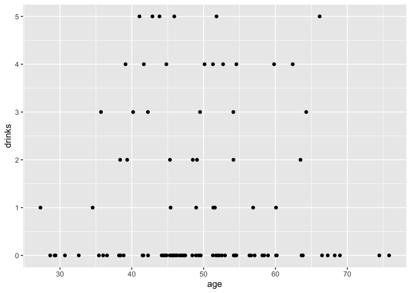
## `geom_smooth()` using formula = 'y ~ x'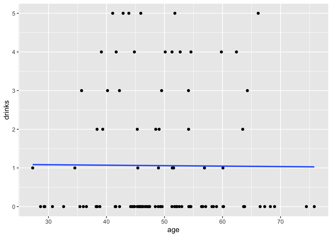
##
## Call:  glm(formula = drinks ~ age, family = poisson(link = "log"), data = drinks)
##
## Coefficients:
## (Intercept)          age
##    0.113739    -0.001131
##
## Degrees of Freedom: 99 Total (i.e. Null);  98 Residual
## Null Deviance:       243
## Residual Deviance: 243   AIC: 349.5
17.3.2 Interpretation
Intercept: The natural log of the mean number of
drinkswhenageis equal to zero is 0.113739.age: The average change in the natural log of the mean number of
drinksfor each one-year increase inageis -0.001131.
## # A tibble: 2 × 5
##   term        estimate std.error statistic p.value
##   <chr>          <dbl>     <dbl>     <dbl>   <dbl>
## 1 (Intercept)    1.12    0.485       0.234   0.815
## 2 age 0.999 0.00970 -0.117 0.907- Participants reported 0.9 times the number of drinks at their last drinking episode for each one-year increase in age.
## [1] 0.057189## [1] 0.056058## [1] -0.001131## [1] 0.9988696This is an incidence rate ratio. Remember that a rate is just the number of events per some specified period of time. In this case, the specified period of time is the same for all participants, so the “missing” time cancels out, and we get a rate ratio.
What’s our null value for a rate ratio?
17.3.3 Count regressand categorical regressor
## [1] 1.06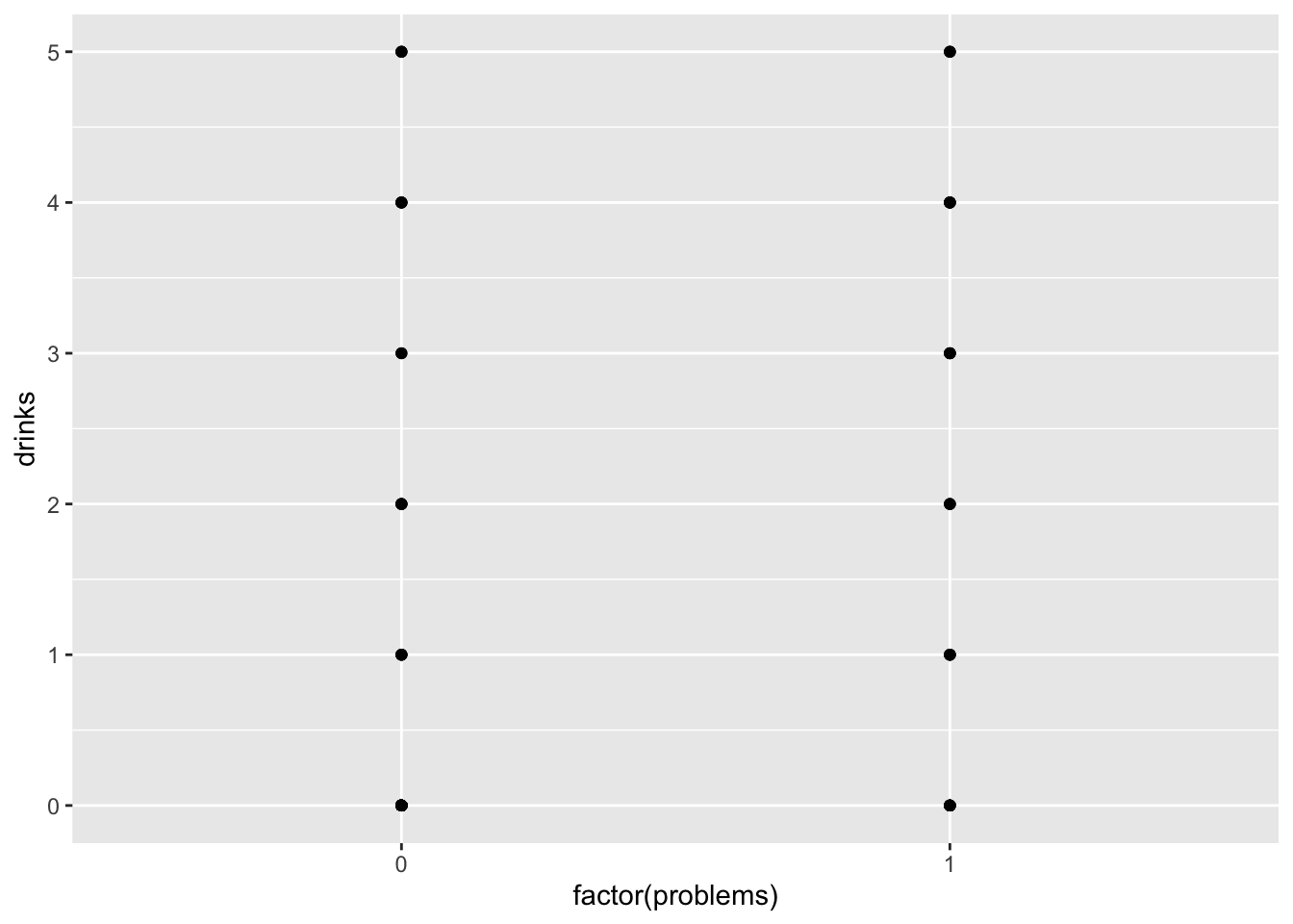
ggplot(drinks, aes(x = factor(problems), y = drinks)) +
geom_jitter(width = 0, height = 0.25, alpha = .5) 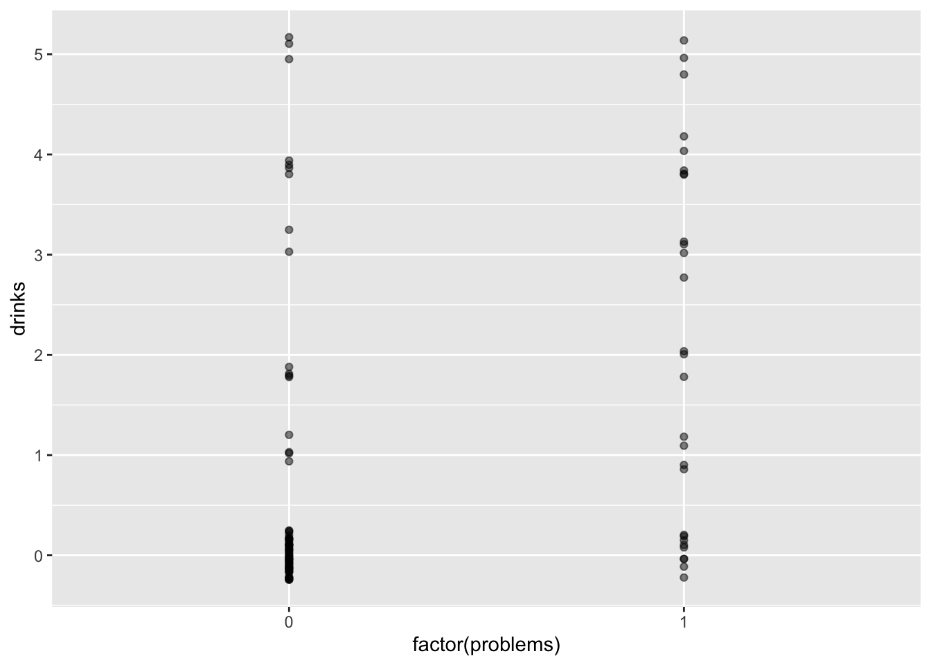
##
## Call:  glm(formula = drinks ~ problems, family = poisson(link = "log"),
##     data = drinks)
##
## Coefficients:
## (Intercept)     problems
##     -0.3848       1.0957
##
## Degrees of Freedom: 99 Total (i.e. Null);  98 Residual
## Null Deviance:       243
## Residual Deviance: 212   AIC: 318.5
17.3.4 Interpretation
Intercept: The natural log of the mean number of
drinkswhenproblemsis equal to zero is -0.3848.problems: The average change in the natural log of the mean of
drinkswhenproblemschanges from zero to one.
## # A tibble: 2 × 5
##   term        estimate std.error statistic      p.value
##   <chr>          <dbl>     <dbl>     <dbl>        <dbl>
## 1 (Intercept)    0.681     0.143     -2.69 0.00706
## 2 problems 2.99 0.195 5.62 0.0000000186- Participants reporting that they had personal problems, drank 2.99 times more drinks at their last drinking episode compared to those who reported no personal problems.
This is an incidence rate ratio. Remember that a rate is just the number of events per some specified period of time. In this case, the specified period of time is the same for all participants, so the “missing” time cancels out, and we get a rate ratio.
17.4 Assumptions
Here are some assumptions of the logistic model to keep in mind.
Natural logarithm of the expected number of events per unit time changes linearly with the predictors
At each level of the predictors, the number of events per unit time has variance equal to the mean
Observations are independent