15 Linear Regression
This chapter is under heavy development and may still undergo significant changes.
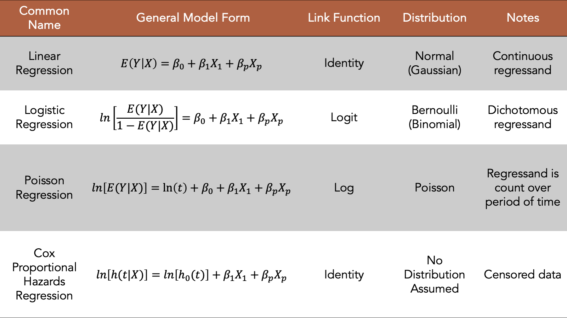
Figure 15.1: Four commonly used generalized linear models.
We introduced regression modeling generally in the introduction to regression analysis chapter. In this chapter, we will discuss fitting linear regression models, a type of generalized linear model, to our data using R. In general, the linear model is a good place to start when the regressand we want to model is continuous. We will begin by loading some useful R packages and simulating some data to fit our model to. We add comments to the code below to help you get a sense for how the values in the simulated data are generated. But please skip over the code if it feels distracting or confusing, as it is not the primary object of our interest right now.
# Load the packages we will need below
library(dplyr, warn.conflicts = FALSE)
library(broom) # Makes glm() results easier to read and work with
library(ggplot2)
library(meantables)
library(freqtables)
# Set the seed for the random number generator so that we can reproduce our results
set.seed(123)
# Set n to equal the number of people we want to simulate. We will use n
# repeatedly in the code below.
n <- 20
# Simulate a data frame with n rows
# The variables in the data frame are generic continuous, categorical, and
# count values. They aren't necessarily intended to represent any real-life
# health-related state or event
df <- tibble(
# Create a continuous regressor containing values selected at random from
# a normal distribution
x_cont = rnorm(n, 10, 1),
# Create a categorical regressor containing values selected at random from
# a binomial distribution with a 0.3 probability of success (i.e.,
# selecting a 1)
x_cat = rbinom(n, 1, .3),
# Create a continuous regressand that has a value that is equal to the value
# of x_cont plus or minus some random variation. The direction of the
# variation is dependent on the value of x_cat.
y_cont = if_else(
x_cat == 0,
x_cont + rnorm(n, 1, 0.1),
x_cont - rnorm(n, 1, 0.1)
),
# Create a categorical regressand that has a value selected at random from
# a binomial distribution. The probability of a successful draw from the
# binomial distribution is dependent on the value of x_cat.
y_cat = if_else(
x_cat == 0,
rbinom(n, 1, .1),
rbinom(n, 1, .5)
),
# Create a regressand that contains count data selected at random from
# a categorical distribution. The probability of a selecting each value from
# the distribution is dependent on the value of x_cat.
y_count = if_else(
x_cat == 0,
sample(1:5, n, TRUE, c(.1, .2, .3, .2, .2)),
sample(1:5, n, TRUE, c(.3, .3, .2, .1, .1))
)
)
# Print the value stored in df to the screen
df## # A tibble: 20 × 5
## x_cont x_cat y_cont y_cat y_count
## <dbl> <int> <dbl> <int> <int>
## 1 9.44 0 10.5 0 5
## 2 9.77 0 10.7 0 2
## 3 11.6 0 12.6 0 5
## 4 10.1 0 11.2 0 3
## 5 10.1 0 11.2 0 4
## 6 11.7 0 12.8 0 2
## 7 10.5 0 11.5 0 3
## 8 8.73 0 9.73 0 4
## 9 9.31 0 10.3 0 1
## 10 9.55 1 8.53 0 1
## 11 11.2 0 12.2 0 3
## 12 10.4 0 11.3 0 2
## 13 10.4 1 9.43 1 1
## 14 10.1 0 11.3 0 4
## 15 9.44 0 10.6 0 1
## 16 11.8 0 12.7 0 2
## 17 10.5 0 11.5 0 2
## 18 8.03 1 7.03 1 2
## 19 10.7 1 9.61 1 5
## 20 9.53 0 10.5 0 415.1 Continuous regressand and continuous regressor
Now that we have some simulated data, we will fit and interpret a few different linear models. We will start by fitting a linear model with a single continuous regressor.
glm(
  y_cont ~ x_cont,                      # Formula
  family = gaussian(link = "identity"), # Family/distribution/Link function
  data   = df                           # Data
)
##
## Call: glm(formula = y_cont ~ x_cont, family = gaussian(link = "identity"),
## data = df)
##
## Coefficients:
## (Intercept) x_cont
## -1.430 1.202
##
## Degrees of Freedom: 19 Total (i.e. Null); 18 Residual
## Null Deviance: 38.79
## Residual Deviance: 12.82 AIC: 53.86This model isn’t the most interesting model to interpret because we are just modeling numbers without any context. However, because we are modeling numbers without any context, we can strip out any unnecessary complexity or biases from our interpretations. Therefore, in a sense, these will be the “purist”, or at least the most general, interpretations of the regression coefficients produced by this type of model. We hope that learning these general interpretations will help us to understand the models, and to more easily interpret more complex models in the future.
15.2 Continuous regressand and categorical regressor
Next, we will fit a linear model with a single categorical regressor. Notice that the formula syntax, the distribution, and the link function are the same for the single categorical regressor as they were for the single continuous predictor. We just swap our x_cont for x_cat in the formula.
glm(
  y_cont ~ x_cat,                       # Formula
  family = gaussian(link = "identity"), # Family/distribution/Link function
  data   = df                           # Data
)
##
## Call: glm(formula = y_cont ~ x_cat, family = gaussian(link = "identity"),
## data = df)
##
## Coefficients:
## (Intercept) x_cat
## 11.287 -2.636
##
## Degrees of Freedom: 19 Total (i.e. Null); 18 Residual
## Null Deviance: 38.79
## Residual Deviance: 16.55 AIC: 58.9815.2.1 Interpretation
Intercept: The mean value of
y_contwhenx_catis equal to zero.x_cat: The change in the mean value of
y_contwhenx_catchanges from zero to one.
Now that we have reviewed the general interpretations, let’s practice using linear regression to explore the relationship between two variables that feel more like a scenario that we may plausibly be interested in.
15.3 Waist circumference and deep abdominal adipose tissue example
“Despres et al. point out that the topography of adipose tissue (AT) is associated with metabolic complications considered as risk factors for cardiovascular disease. It is important, they state, to measure the amount of of intraabdominal AT as part of the evaluation of the cardiovascular-disease risk of an individual. Computed tomography (CT), the only available technique that precisely and reliably measures the amount of deep abdominal AT, however, is costly and requires irradiation of the subject. In addition, the technique is not available to many physicians. Depres and his colleagues conducted a study to develop equations to predict the amount of deep abdominal AT from simple anthropometric measurements. Their subjects were men between the ages of 18 and 42 years who were free from metabolic disease that would require treatment. Among the measurements taken on each subject were deep abdominal AT obtained by CT and waist circumference. A question of interest is how well one can predict and estimate deep abdominal AT from knowledge of waist circumference.”5
We will start by simulating some data to roughly match the scenario above.
set.seed(123)
n <- 100
daat_waist <- tibble(
  waist    = rnorm(n, 39, 2),
  waist_c  = waist - 39,
  beta1    = rnorm(n, 3.45, 0.2),
  daat_bar = rnorm(n, 101, 8),
  daat     = daat_bar + (beta1 * waist_c)
)
daat_waist
## # A tibble: 100 × 5
## waist waist_c beta1 daat_bar daat
## <dbl> <dbl> <dbl> <dbl> <dbl>
## 1 37.9 -1.12 3.31 119. 115.
## 2 38.5 -0.460 3.50 111. 110.
## 3 42.1 3.12 3.40 98.9 109.
## 4 39.1 0.141 3.38 105. 106.
## 5 39.3 0.259 3.26 97.7 98.5
## 6 42.4 3.43 3.44 97.2 109.
## 7 39.9 0.922 3.29 94.7 97.7
## 8 36.5 -2.53 3.12 96.2 88.4
## 9 37.6 -1.37 3.37 114. 110.
## 10 38.1 -0.891 3.63 101. 97.3
## # ℹ 90 more rowsNow, let’s explore the relationship between waist circumference and deep abdominal adipose tissue in our simulated data.
15.3.1 Continuous regressor (waist circumference)
What is the average waist circumference?
## [1] 39.18081What is the average value of deep abdominal adipose tissue?
## [1] 102.5663What does the relationship between deep abdominal adipose tissue and waist circumference look like as a scatter plot?
ggplot(daat_waist, aes(x = waist, y = daat)) +
  geom_point() +
  ylab("Deep abdominal adipose tissue") +
  xlab("Waist circumference") +
  theme_bw()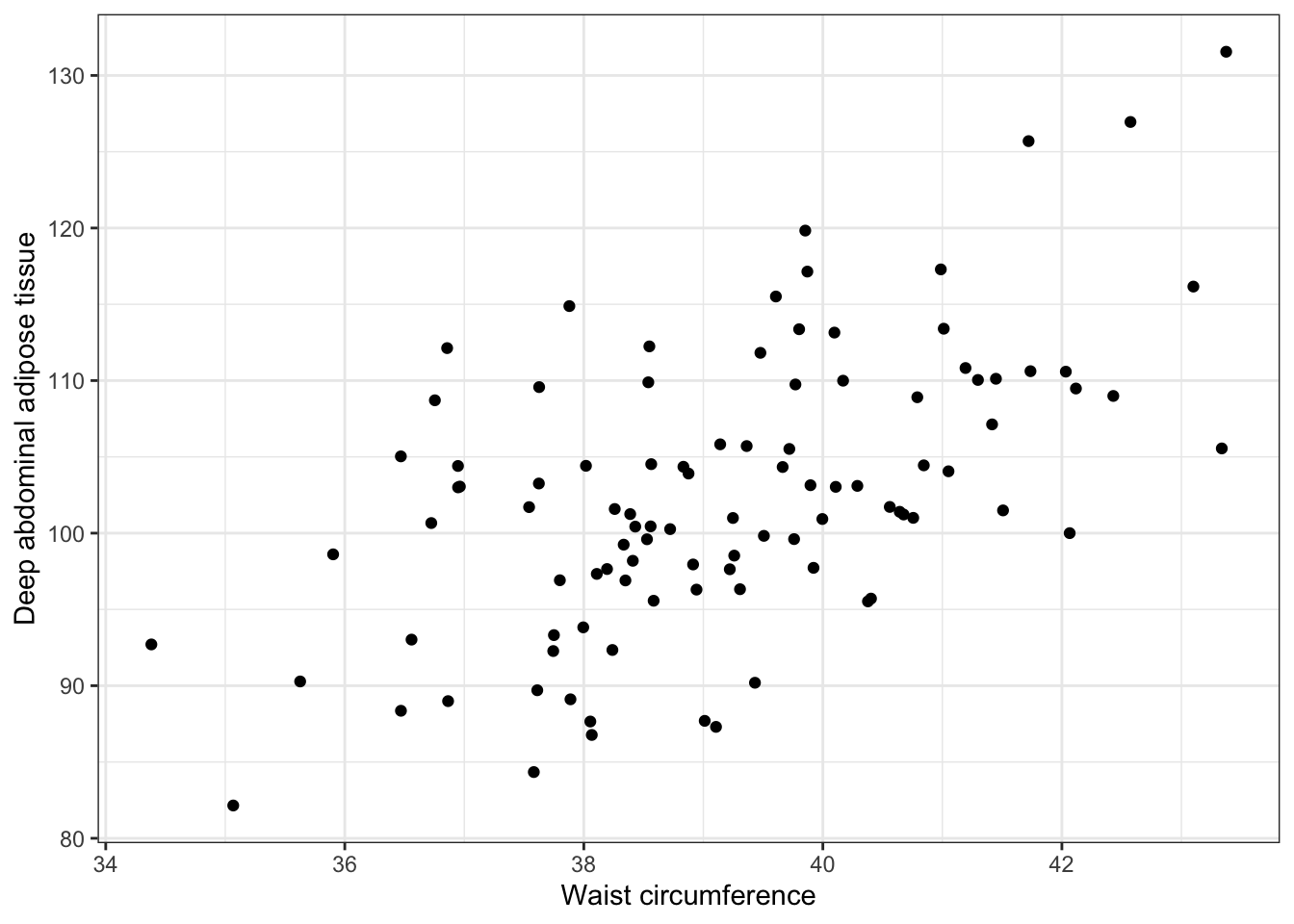
What is the relationship between deep abdominal adipose tissue (regressand) and waist circumference (regressor)?
##
## Call:  glm(formula = daat ~ waist, family = gaussian(link = "identity"),
##     data = daat_waist)
##
## Coefficients:
## (Intercept)        waist
##      -9.580        2.862
##
## Degrees of Freedom: 99 Total (i.e. Null);  98 Residual
## Null Deviance:       8404
## Residual Deviance: 5701  AIC: 694.1
15.3.1.1 Interpretation
Intercept: The mean value of deep abdominal adipose tissue when waist circumference is 0 is -9.580.
waist: The average change in deep abdominal adipose tissue for each one inch increase in waist circumference is 2.86.
And we can add this information to our plot.
ggplot(daat_waist, aes(x = waist, y = daat)) +
  geom_point() +
  geom_abline(intercept = -9.580, slope = 2.862, color = "red", linetype = "dashed") +
  ylab("Deep abdominal adipose tissue") +
  xlab("Waist circumference") +
  theme_bw()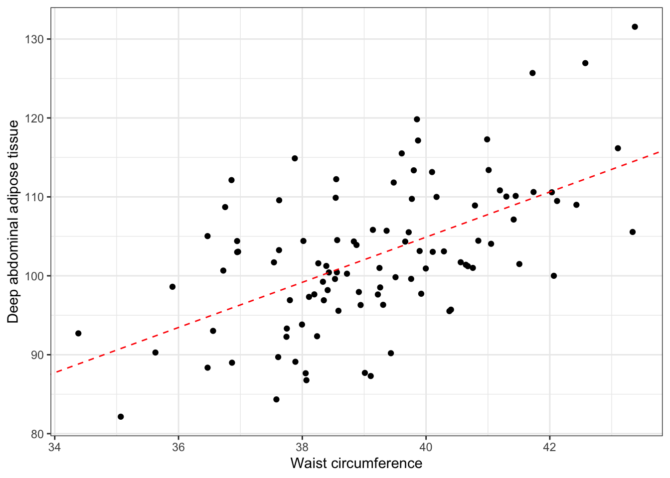
15.3.2 Categorical regressor (large waist)
daat_waist <- daat_waist %>%
  mutate(
    large_waist   = if_else(waist < mean(waist), 0, 1),
    large_waist_f = factor(large_waist, 0:1, c("No", "Yes"))
  )
daat_waist
## # A tibble: 100 × 7
## waist waist_c beta1 daat_bar daat large_waist large_waist_f
## <dbl> <dbl> <dbl> <dbl> <dbl> <dbl> <fct>
## 1 37.9 -1.12 3.31 119. 115. 0 No
## 2 38.5 -0.460 3.50 111. 110. 0 No
## 3 42.1 3.12 3.40 98.9 109. 1 Yes
## 4 39.1 0.141 3.38 105. 106. 0 No
## 5 39.3 0.259 3.26 97.7 98.5 1 Yes
## 6 42.4 3.43 3.44 97.2 109. 1 Yes
## 7 39.9 0.922 3.29 94.7 97.7 1 Yes
## 8 36.5 -2.53 3.12 96.2 88.4 0 No
## 9 37.6 -1.37 3.37 114. 110. 0 No
## 10 38.1 -0.891 3.63 101. 97.3 0 No
## # ℹ 90 more rows## # A tibble: 2 × 11
## response_var group_var group_cat n mean sd sem lcl ucl min max
## <chr> <chr> <fct> <int> <dbl> <dbl> <dbl> <dbl> <dbl> <dbl> <dbl>
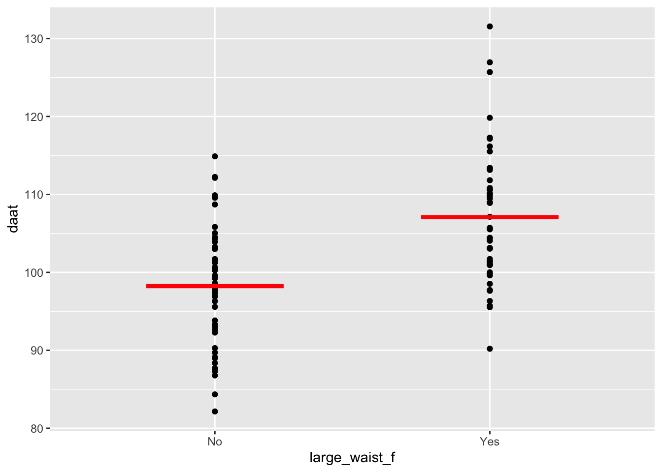
## 1 daat large_waist_f No 51 98.2 7.71 1.08 96.1 100. 82.1 115.
## 2 daat large_waist_f Yes 49 107. 8.51 1.22 105. 110. 90.2 132.ggplot(daat_waist, aes(x = large_waist_f, y = daat)) +
geom_point() +
geom_segment(
aes(x = c(0.75, 1.75), y = mean, xend = c(1.25, 2.25), yend = mean),
linewidth = 1.5, color = "red", data = daat_by_large_f
)
What is the relationship between deep abdominal adipose tissue (regressand) and tall (regressor)?
##
## Call:  glm(formula = daat ~ large_waist_f, family = gaussian(link = "identity"),
##     data = daat_waist)
##
## Coefficients:
##      (Intercept)  large_waist_fYes
##           98.228             8.854
##
## Degrees of Freedom: 99 Total (i.e. Null);  98 Residual
## Null Deviance:       8404
## Residual Deviance: 6445  AIC: 706.4
15.3.2.1 Interpretation
Intercept: The mean value of deep abdominal adipose tissue among people who are not tall is equal to 98.228.
large_waist_fYes: The average change in deep abdominal adipose tissue for people with a large waste circumference compared to people with a small waste circumference is 8.854.
## [1] 107.082